Скачать с ютуб How To Highlight Rows Based On Specific Text In Excel в хорошем качестве

How To Highlight Rows Based On Specific Text In Excel

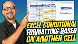
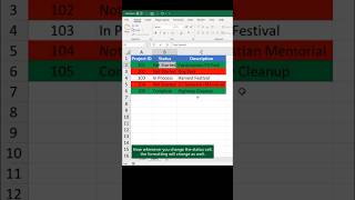
How To Highlight Rows Based On Specific Text In Excel In this excel tutorial, I’ll explain an interesting way to highlight row if cell contains specific text. You can also highlight rows in excel based on value within your selection or if the entire row. I’ll be using conditional formatting to solve this. If you apply the conditional formatting to a selection then it will highlight rows within that selection and if you apply this to entire worksheet then it will mark the entire row. Our challenge here is to create a dynamic highlight option that we create once will work until we remove it. In this case I’ve highlighted rows based on a specific text that I have on another cell. This dynamic formatting checks if the specific text that is in the cell we have selected matches or not. If it matches then the entire row will be highlighted with the color we select and if not, then nothing happens. This tutorial will be very helpful if you have a transaction list and you want to locate or highlight every transaction from a specific buyer of vendor. Now let’s follow the steps below to apply conditional formatting if cell contains specific text and highlight it with pre-defined color. Step 1: Select the entire worksheet (To highlight entire row) or a selection where you’ll have data (To highlight rows within that selection) Step 2: Click on “conditional formatting” and then “new rule” Step 3: Click on “Select formula to specify which cells to format” Step 4: Now write the first cell no. of the column where you need to match your data then write = (Equal to) and then the specific text or cell number where you’ll have your specific text. Step 5: Click on format and select the highlight color from there and click Ok Twice. Done. This is how we change of a row color based on a text value in another cell. Notes: In step 4 you need to write the cell number of the column where you need to check specific text will have to write in this format $C2 not $C$2 or C2. All you need to remember is that $C means the column number is fixed, it will not change. And the row number here will change and check if any cell has the text, you specified and then take action. #HighlightRow #BasedOnCellValue Thanks for watching. ------------------------------------------------------------------------------------------------------------- Support the channel with as low as $5   / excel10tutorial   ------------------------------------------------------------------------------------------------------------- Please subscribe to #excel10tutorial https://goo.gl/uL8fqQ Here goes the most recent video of the channel: https://bit.ly/2UngIwS Playlists: Advance Excel Tutorial: https://goo.gl/ExYy7v Excel Tutorial for Beginners: https://goo.gl/UDrDcA Excel Case: https://goo.gl/xiP3tv Combine Workbook & Worksheets: https://bit.ly/2Tpf7DB All About Comments in Excel: https://bit.ly/excelcomments Excel VBA Programming Course: http://bit.ly/excelvbacourse Social media: Facebook:   / excel10tutorial   Twitter:   / excel10tutorial   Blogger: https://excel10tutorial.blogspot.com Tumblr:   / excel10tutorial   Instagram:   / excel_10_tutorial   Hubpages: https://hubpages.com/@excel10tutorial Quora: https://bit.ly/3bxB8JG